Example Quarto manuscript

1 Introduction
“Literate programming” is a style of programming that uses computational notebooks to weave together code, explanatory text, data and results into a single document, enhancing scientific communication and computational reproducibility.1–3 (These references were added into the document using RStudio’s integration with the open-source Zotero reference manager4 plus the Better BibTeX Zotero plugin.)
Several platforms for creating such documents exist.5 Typically, these documents interleave code and text ‘blocks’ to build a computational narrative. But some, including R Markdown, Observable, and the Jupyter Book extension to the Jupyter ecosystem, also allow authors to include and execute code “inline” – that is, within the text itself.
The newest entry to this toolset is Quarto. “an open-source scientific and technical publishing system built on Pandoc.” See https://quarto.org/docs/guide/ for a guide to authoring in Quarto.
To learn more about executable manuscripts, check out our Nature feature, published 28 February 2022.
Whichever you use, these platforms make it possible to create fully executable manuscripts in which the document itself computes and inserts values and figures into the text rather than requiring authors to input them manually. This is in many ways the ‘killer feature’ of computed manuscripts: it circumvents the possibility that the author will enter an incorrect number, or forget to update a figure or value should new data arise. Among other uses, that allows authors to automatically time-stamp their documents, or insert the current version number of the software they use into their methods. For instance, this document was built at 04 Aug 2022 14:24:24 MST and uses the following R packages: {tidyverse} ver. 1.3.0 and {ggbeeswarm} ver. 0.6.0.
In this manuscript, created in RStudio using Quarto, we will demonstrate a more practical example. (An Observable version is also available.)
2 Results
2.1 Inline computation
Imagine we are analyzing data from a clinical trial. We have grouped subjects in three bins and measured the concentration of some metabolite. (These data are simulated.)
Rather than analyzing those data and then copying the results into our manuscript, we can use the programming language R to do that in the manuscript itself. Simply enclose the code inside backticks, with the letter r. For instance, we could calculate the circumference and area of a circle, using the ObservableJS library to make things interactive:
\[A = \pi r^2, C = 2 \pi r\]
Plugging in the radius r = , A = and C = .
Returning to our dataset, we can count the rows in our table to determine the number of samples, and insert that into the text. Thus, we have 99 (simulated) subjects in our study (see Table 1; see R/mock_data.R in the GitHub repository for code to generate a mock dataset). Note that the tables, figures and sections in this document are numbered automatically.
The average metabolite concentration in this dataset is 185.36 (range: 78 to 298). We have 32 subjects in Group 1, 43 subjects in Group 2, and 24 in Group 3. (The numbers in bold face type throughout this document are computed values.)
2.2 Incorporating new data
Now suppose we get another tranche of data (Table 2). There are 60 subjects in this new dataset, with an average concentration of 185.13 (range: 77 to 299).
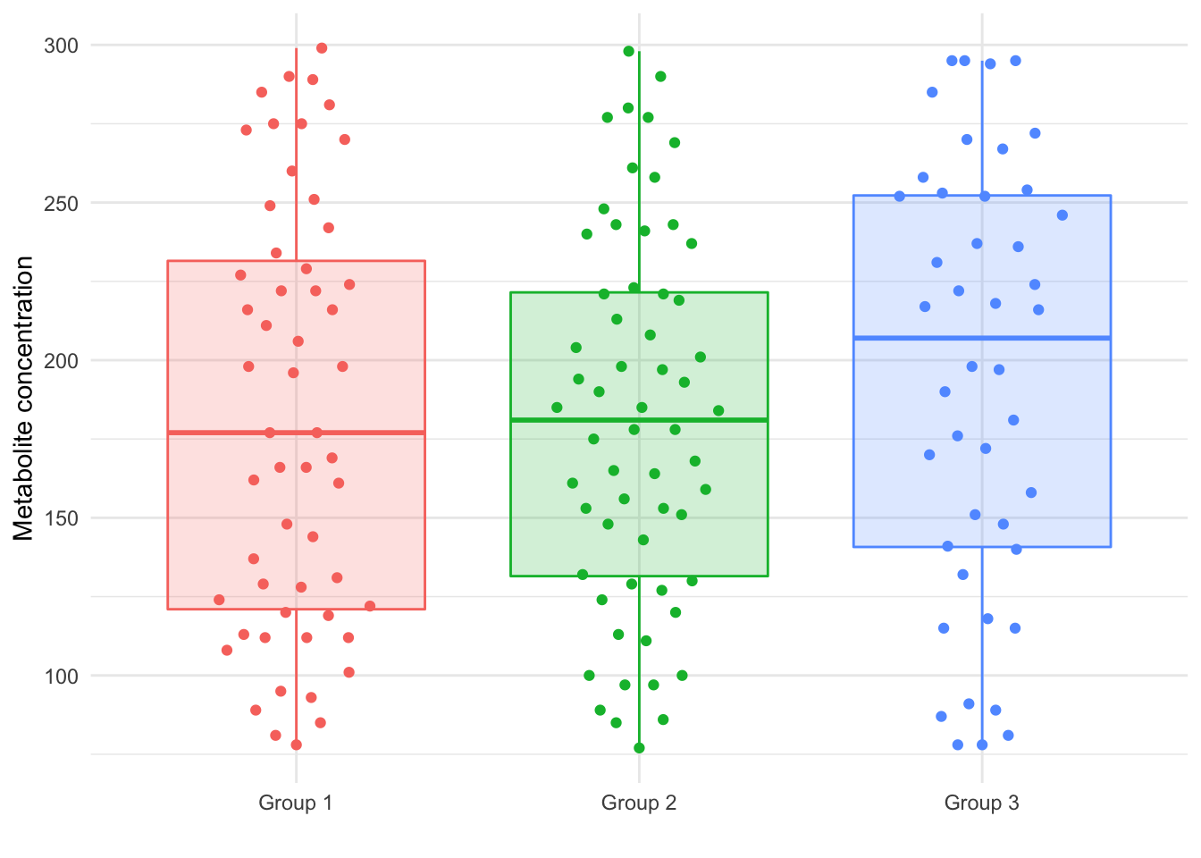
Combining the two datasets, we have a total of 159 subjects with an average metabolite concentration of 185.28 (range: 77 to 299). We now have 55 subjects in Group 1, 60 in Group 2, and 44 in Group 3. The concentration distribution for each group in this joint dataset is shown graphically in Figure 1.
3 Importing a child document
Authors can break long manuscripts into more manageable pieces by placing each chapter or section in their own Markdown file and using Quarto’s child option. Though most of the text (and code) in this document is contained in the file index.qmd, the text for this section comes from child_doc.qmd. Citations that are created in the child automatically get inserted into the final document, making it possible to create a single, unified bibliography. For instance, here’s a reference for the R Markdown Cookbook.6
In this child document, we’ll add a third set of numbers to our growing dataset (Table 3); note that the table, figure and section numbering in this child document matches that of the larger manuscript).
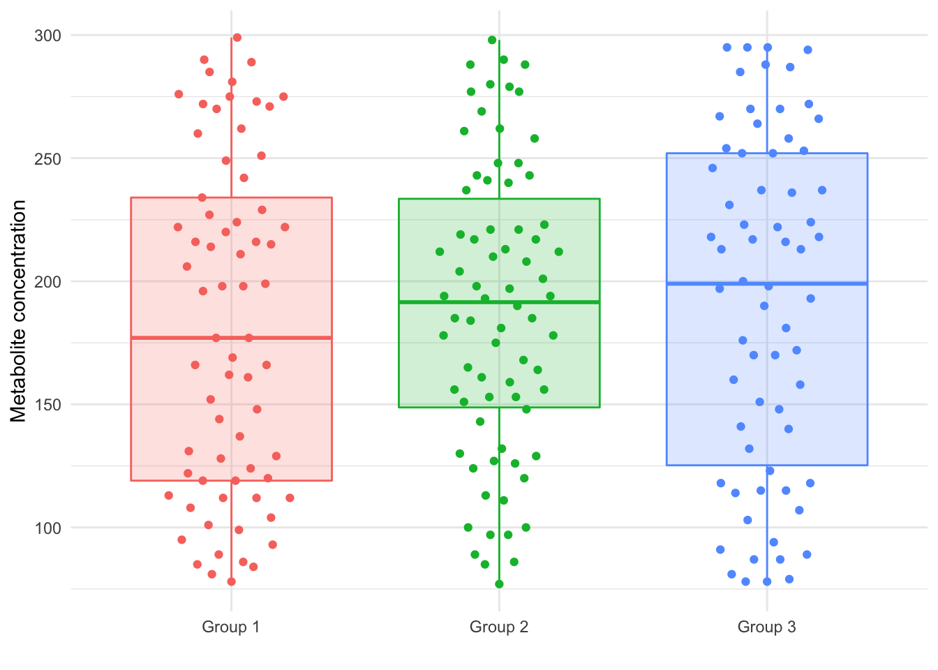
The new dataset describes 50 samples. Folding them into our existing data gives us 209 subjects, with 69 in Group 1, 74 in Group 2, and 66 in Group 3. The new concentration distribution is shown graphically in Figure 2.
| ID | Class | Conc | | | ID | Class | Conc | | | ID | Class | Conc |
|---|---|---|---|---|---|---|---|---|---|---|
| ID_1 | Group 2 | 153 | | | ID_34 | Group 2 | 221 | | | ID_67 | Group 3 | 148 |
| ID_2 | Group 1 | 224 | | | ID_35 | Group 1 | 112 | | | ID_68 | Group 1 | 281 |
| ID_3 | Group 2 | 127 | | | ID_36 | Group 3 | 246 | | | ID_69 | Group 3 | 295 |
| ID_4 | Group 2 | 194 | | | ID_37 | Group 2 | 190 | | | ID_70 | Group 2 | 111 |
| ID_5 | Group 1 | 251 | | | ID_38 | Group 1 | 177 | | | ID_71 | Group 2 | 132 |
| ID_6 | Group 1 | 81 | | | ID_39 | Group 1 | 148 | | | ID_72 | Group 2 | 261 |
| ID_7 | Group 2 | 100 | | | ID_40 | Group 2 | 290 | | | ID_73 | Group 1 | 122 |
| ID_8 | Group 1 | 270 | | | ID_41 | Group 2 | 151 | | | ID_74 | Group 2 | 124 |
| ID_9 | Group 2 | 100 | | | ID_42 | Group 2 | 159 | | | ID_75 | Group 1 | 234 |
| ID_10 | Group 1 | 161 | | | ID_43 | Group 2 | 113 | | | ID_76 | Group 2 | 184 |
| ID_11 | Group 3 | 158 | | | ID_44 | Group 1 | 249 | | | ID_77 | Group 3 | 272 |
| ID_12 | Group 3 | 118 | | | ID_45 | Group 1 | 124 | | | ID_78 | Group 1 | 242 |
| ID_13 | Group 2 | 143 | | | ID_46 | Group 3 | 87 | | | ID_79 | Group 2 | 277 |
| ID_14 | Group 2 | 258 | | | ID_47 | Group 1 | 166 | | | ID_80 | Group 3 | 236 |
| ID_15 | Group 3 | 224 | | | ID_48 | Group 1 | 196 | | | ID_81 | Group 1 | 101 |
| ID_16 | Group 3 | 254 | | | ID_49 | Group 1 | 112 | | | ID_82 | Group 3 | 218 |
| ID_17 | Group 3 | 190 | | | ID_50 | Group 1 | 289 | | | ID_83 | Group 2 | 130 |
| ID_18 | Group 2 | 148 | | | ID_51 | Group 2 | 161 | | | ID_84 | Group 1 | 128 |
| ID_19 | Group 1 | 89 | | | ID_52 | Group 3 | 270 | | | ID_85 | Group 3 | 252 |
| ID_20 | Group 2 | 89 | | | ID_53 | Group 2 | 237 | | | ID_86 | Group 1 | 198 |
| ID_21 | Group 3 | 253 | | | ID_54 | Group 2 | 280 | | | ID_87 | Group 1 | 169 |
| ID_22 | Group 3 | 231 | | | ID_55 | Group 2 | 175 | | | ID_88 | Group 2 | 185 |
| ID_23 | Group 1 | 112 | | | ID_56 | Group 2 | 223 | | | ID_89 | Group 1 | 216 |
| ID_24 | Group 2 | 277 | | | ID_57 | Group 3 | 295 | | | ID_90 | Group 2 | 185 |
| ID_25 | Group 2 | 197 | | | ID_58 | Group 1 | 275 | | | ID_91 | Group 2 | 97 |
| ID_26 | Group 2 | 208 | | | ID_59 | Group 2 | 120 | | | ID_92 | Group 2 | 165 |
| ID_27 | Group 2 | 193 | | | ID_60 | Group 1 | 78 | | | ID_93 | Group 3 | 89 |
| ID_28 | Group 3 | 141 | | | ID_61 | Group 3 | 78 | | | ID_94 | Group 2 | 221 |
| ID_29 | Group 1 | 206 | | | ID_62 | Group 3 | 140 | | | ID_95 | Group 1 | 162 |
| ID_30 | Group 2 | 168 | | | ID_63 | Group 3 | 294 | | | ID_96 | Group 1 | 131 |
| ID_31 | Group 2 | 298 | | | ID_64 | Group 3 | 295 | | | ID_97 | Group 1 | 93 |
| ID_32 | Group 1 | 144 | | | ID_65 | Group 3 | 285 | | | ID_98 | Group 2 | 240 |
| ID_33 | Group 2 | 241 | | | ID_66 | Group 2 | 129 | | | ID_99 | Group 2 | 86 |
| ID | Class | Conc | | | ID | Class | Conc | | | ID | Class | Conc |
|---|---|---|---|---|---|---|---|---|---|---|
| ID_100 | Group 2 | 219 | | | ID_120 | Group 2 | 85 | | | ID_140 | Group 2 | 77 |
| ID_101 | Group 2 | 243 | | | ID_121 | Group 3 | 181 | | | ID_141 | Group 1 | 299 |
| ID_102 | Group 2 | 213 | | | ID_122 | Group 3 | 216 | | | ID_142 | Group 3 | 222 |
| ID_103 | Group 1 | 177 | | | ID_123 | Group 1 | 222 | | | ID_143 | Group 1 | 85 |
| ID_104 | Group 3 | 197 | | | ID_124 | Group 3 | 252 | | | ID_144 | Group 1 | 273 |
| ID_105 | Group 2 | 198 | | | ID_125 | Group 1 | 166 | | | ID_145 | Group 3 | 115 |
| ID_106 | Group 1 | 120 | | | ID_126 | Group 2 | 204 | | | ID_146 | Group 1 | 290 |
| ID_107 | Group 3 | 170 | | | ID_127 | Group 2 | 243 | | | ID_147 | Group 2 | 269 |
| ID_108 | Group 3 | 78 | | | ID_128 | Group 3 | 198 | | | ID_148 | Group 2 | 97 |
| ID_109 | Group 1 | 129 | | | ID_129 | Group 1 | 119 | | | ID_149 | Group 1 | 229 |
| ID_110 | Group 1 | 137 | | | ID_130 | Group 1 | 198 | | | ID_150 | Group 3 | 176 |
| ID_111 | Group 3 | 217 | | | ID_131 | Group 3 | 151 | | | ID_151 | Group 2 | 164 |
| ID_112 | Group 1 | 227 | | | ID_132 | Group 3 | 115 | | | ID_152 | Group 3 | 172 |
| ID_113 | Group 3 | 81 | | | ID_133 | Group 3 | 237 | | | ID_153 | Group 1 | 222 |
| ID_114 | Group 2 | 248 | | | ID_134 | Group 2 | 178 | | | ID_154 | Group 1 | 285 |
| ID_115 | Group 1 | 211 | | | ID_135 | Group 1 | 275 | | | ID_155 | Group 2 | 153 |
| ID_116 | Group 1 | 113 | | | ID_136 | Group 2 | 178 | | | ID_156 | Group 3 | 132 |
| ID_117 | Group 1 | 216 | | | ID_137 | Group 3 | 267 | | | ID_157 | Group 2 | 156 |
| ID_118 | Group 3 | 91 | | | ID_138 | Group 1 | 95 | | | ID_158 | Group 1 | 260 |
| ID_119 | Group 3 | 258 | | | ID_139 | Group 1 | 108 | | | ID_159 | Group 2 | 201 |
| ID | Class | Conc | | | ID | Class | Conc | | | ID | Class | Conc |
|---|---|---|---|---|---|---|---|---|---|---|
| ID_160 | Group 2 | 210 | | | ID_177 | Group 2 | 288 | | | ID_194 | Group 3 | 123 |
| ID_161 | Group 3 | 107 | | | ID_178 | Group 1 | 262 | | | ID_195 | Group 2 | 212 |
| ID_162 | Group 2 | 262 | | | ID_179 | Group 2 | 217 | | | ID_196 | Group 1 | 99 |
| ID_163 | Group 1 | 215 | | | ID_180 | Group 3 | 87 | | | ID_197 | Group 3 | 264 |
| ID_164 | Group 1 | 220 | | | ID_181 | Group 3 | 266 | | | ID_198 | Group 2 | 279 |
| ID_165 | Group 3 | 288 | | | ID_182 | Group 3 | 79 | | | ID_199 | Group 2 | 126 |
| ID_166 | Group 3 | 287 | | | ID_183 | Group 1 | 152 | | | ID_200 | Group 1 | 276 |
| ID_167 | Group 3 | 213 | | | ID_184 | Group 3 | 223 | | | ID_201 | Group 3 | 213 |
| ID_168 | Group 1 | 84 | | | ID_185 | Group 3 | 118 | | | ID_202 | Group 2 | 212 |
| ID_169 | Group 3 | 160 | | | ID_186 | Group 1 | 214 | | | ID_203 | Group 1 | 104 |
| ID_170 | Group 2 | 194 | | | ID_187 | Group 3 | 200 | | | ID_204 | Group 1 | 199 |
| ID_171 | Group 1 | 119 | | | ID_188 | Group 1 | 271 | | | ID_205 | Group 1 | 272 |
| ID_172 | Group 3 | 218 | | | ID_189 | Group 3 | 237 | | | ID_206 | Group 1 | 86 |
| ID_173 | Group 2 | 217 | | | ID_190 | Group 3 | 170 | | | ID_207 | Group 2 | 181 |
| ID_174 | Group 3 | 103 | | | ID_191 | Group 2 | 156 | | | ID_208 | Group 3 | 114 |
| ID_175 | Group 3 | 94 | | | ID_192 | Group 2 | 288 | | | ID_209 | Group 2 | 248 |
| ID_176 | Group 3 | 270 | | | ID_193 | Group 3 | 193 | | |
4 Colophon
This manuscript was built at 04 Aug 2022 14:24:28 MST using the following computational environment and dependencies:
R version 4.0.4 (2021-02-15)
Platform: x86_64-apple-darwin17.0 (64-bit)
Running under: macOS Big Sur 10.16

Matrix products: default
BLAS:   /Library/Frameworks/R.framework/Versions/4.0/Resources/lib/libRblas.dylib
LAPACK: /Library/Frameworks/R.framework/Versions/4.0/Resources/lib/libRlapack.dylib

locale:
[1] en_US.UTF-8/en_US.UTF-8/en_US.UTF-8/C/en_US.UTF-8/en_US.UTF-8

attached base packages:
[1] stats     graphics  grDevices utils     datasets  methods   base

other attached packages:
 [1] ggbeeswarm_0.6.0 forcats_0.5.1    stringr_1.4.0    dplyr_1.0.8
 [5] purrr_0.3.4      readr_2.1.1      tidyr_1.1.3      tibble_3.1.6
 [9] ggplot2_3.3.5    tidyverse_1.3.0

loaded via a namespace (and not attached):
 [1] Rcpp_1.0.7        lubridate_1.8.0   assertthat_0.2.1  digest_0.6.29
 [5] utf8_1.2.2        R6_2.5.1          cellranger_1.1.0  backports_1.2.1
 [9] reprex_2.0.1      evaluate_0.14     highr_0.9         httr_1.4.2
[13] pillar_1.6.4      rlang_1.0.2       readxl_1.3.1      rstudioapi_0.13
[17] rmarkdown_2.13    labeling_0.4.2    htmlwidgets_1.5.4 bit_4.0.4
[21] munsell_0.5.0     broom_0.7.6       compiler_4.0.4    vipor_0.4.5
[25] modelr_0.1.8      xfun_0.30         pkgconfig_2.0.3   htmltools_0.5.2
[29] tidyselect_1.1.1  fansi_1.0.0       crayon_1.4.2      tzdb_0.2.0
[33] dbplyr_2.1.0      withr_2.4.3       grid_4.0.4        jsonlite_1.8.0
[37] gtable_0.3.0      lifecycle_1.0.1   DBI_1.1.1         magrittr_2.0.2
[41] scales_1.1.1      cli_3.1.0         stringi_1.7.6     vroom_1.5.7
[45] farver_2.1.0      fs_1.5.2          xml2_1.3.3        ellipsis_0.3.2
[49] generics_0.1.1    vctrs_0.3.8       tools_4.0.4       bit64_4.0.5
[53] glue_1.6.0        beeswarm_0.4.0    hms_1.1.1         parallel_4.0.4
[57] fastmap_1.1.0     yaml_2.3.5        colorspace_2.0-0  rvest_1.0.2
[61] knitr_1.37        haven_2.3.1
The current Git commit details are:
[aaf04f9] 2022-08-04: Add TOC and pub date